Modeling
The purpose of Spectacle is to provide a descriptive model of spectral data, where each absorption or emission feature is characterized by an informative Voigt profile. To that end, there are several ways in which users can generate this model to more perfectly match their data, or the data they wish to create.
Defining output data
Support for three different types of output data exists: flux,
flux_decrement, and optical_depth. This indicates the type of data that
will be outputted when the model is run. Output type can be specified upon
creation of a spectacle.modeling.Spectral1D object:
spec_mod = Spectral1D("HI1216", output='optical_depth')
Spectacle internally deals in optical depth space, and optical depth information is transformed into flux as a step in the compound model.
For flux transformations:
And for flux decrement transformations:
All output types use the continuum information when depositing
absorption or emission data into the dispersion bins. Likewise, flux and
flux_decrement will generate results that may be saturated.
>>> from astropy import units as u
>>> import numpy as np
>>> from matplotlib import pyplot as plt
>>> from spectacle.modeling import Spectral1D, OpticalDepth1D
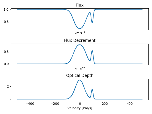
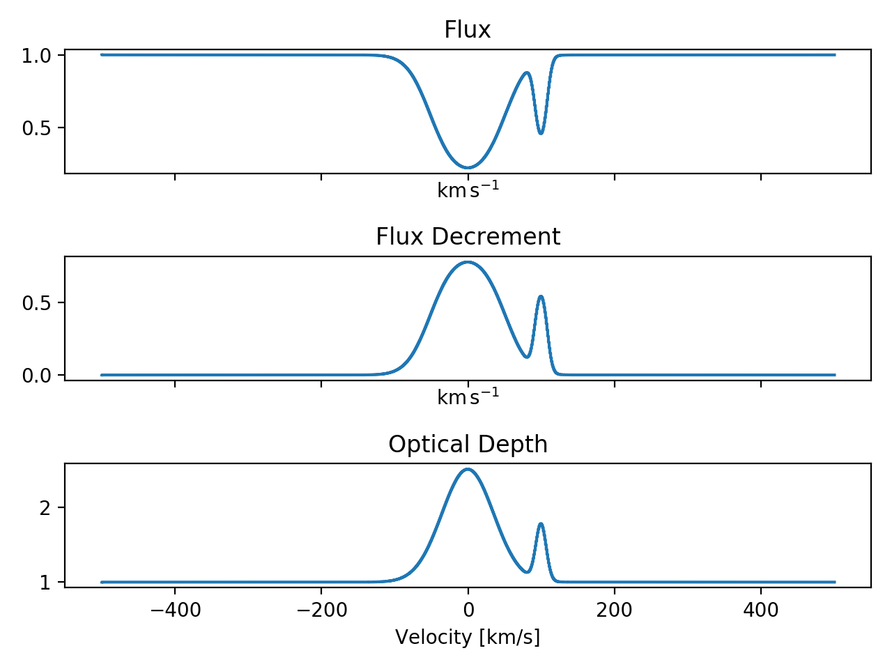
>>> line = OpticalDepth1D("HI1216", v_doppler=50 * u.km/u.s, column_density=14)
>>> line2 = OpticalDepth1D("HI1216", delta_v=100 * u.km/u.s)
>>> spec_mod = Spectral1D([line, line2], continuum=1, output='flux')
>>> x = np.linspace(-500, 500, 1000) * u.Unit('km/s')
>>> flux = spec_mod(x)
>>> flux_dec = spec_mod.as_flux_decrement(x)
>>> tau = spec_mod.as_optical_depth(x)
>>> f, (ax1, ax2, ax3) = plt.subplots(3, 1, sharex=True)
>>> ax1.set_title("Flux")
>>> ax1.step(x, flux)
>>> ax2.set_title("Flux Decrement")
>>> ax2.step(x, flux_dec)
>>> ax3.set_title("Optical Depth")
>>> ax3.step(x, tau)
>>> ax3.set_xlabel('Velocity [km/s]')
>>> f.tight_layout()
(Source code, png, hires.png, pdf)

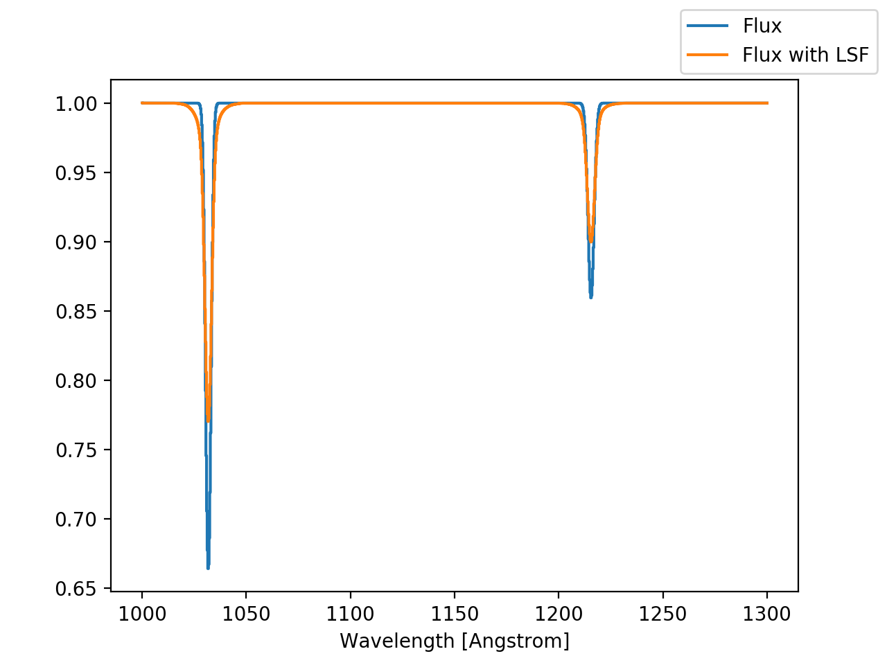
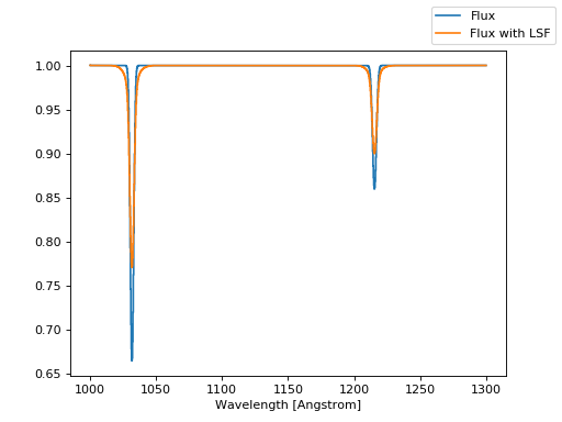
Applying line spread functions
LSFs can be added to the Spectral1D model to
generate data that more appropriately matches what one might expect from an
instrument like, e.g., HST COS
>>> from astropy import units as u
>>> import numpy as np
>>> from matplotlib import pyplot as plt
>>> from spectacle.modeling import Spectral1D, OpticalDepth1D
>>> line1 = OpticalDepth1D("HI1216", v_doppler=500 * u.km/u.s, column_density=14)
>>> line2 = OpticalDepth1D("OVI1032", v_doppler=500 * u.km/u.s, column_density=15)
LSFs can either be applied directly during spectrum model creation:
>>> spec_mod_with_lsf = Spectral1D([line1, line2], continuum=1, lsf='cos', output='flux')
or they can be applied after the fact:
>>> spec_mod = Spectral1D([line1, line2], continuum=1, output='flux')
>>> spec_mod_with_lsf = spec_mod.with_lsf('cos')
>>> x = np.linspace(1000, 1300, 1000) * u.Unit('Angstrom')
>>> f, ax = plt.subplots()
>>> ax.step(x, spec_mod(x), label="Flux")
>>> ax.step(x, spec_mod_with_lsf(x), label="Flux with LSF")
>>> ax.set_xlabel("Wavelength [Angstrom]")
>>> f.legend(loc=0)
(Source code, png, hires.png, pdf)
Supplying custom LSF kernels
Spectacle provides two built-in LSF kernels: the HST COS kernel, and a Gaussian
kernel. Both can be applied by simply passing in a string, and in the latter
case, also supplying an additional stddev keyword argument:
.. code-block:: python
spec_mod = Spectral1D(“HI1216”, continuum=1, lsf=’cos’) spec_mod = Spectral1D(“HI1216”, continuum=1, lsf=’gaussian’, stddev=15)
Users may also supply their own kernels, or any
Astropy 1D kernel.
The only restriction is that kernels must be a subclass of either
LSFModel, or Kernel1D.
from astropy.convolution import Box1DKernel
kernel = Box1DKernel(width=10)

spec_mod_with_lsf = Spectral1D([line1, line2], continuum=1, lsf=kernel, output='flux')
Converting dispersions
Spectacle supports dispersions in either wavelength space or velocity space, and will implicitly deal with conversions internally as necessary. Conversion to velocity space is calculated using the relativistic doppler equation
This of course makes the assumption that observed redshift is due to relativistic effects along the light of sight. At higher redshifts, however, the predominant source of observed redshift is due to the cosmological expansion of space, and not the source’s velocity with respect to the observer.
It is possible to set the approximation used in wavelength/frequency to velocity conversions for Spectacle. Aside from the default relativistic calculation, users can choose the “optical definition”
or the “radio definition”
This can be done upon instantiation of the
Spectral1D model:
spec_mod = Spectral1D("HI1216", continuum=1, z=0, velocity_convention='optical')
The velocity_convention keyword supports one of either relativisitic,
optical, or radio to indiciate the definition to be used in internal
conversions.
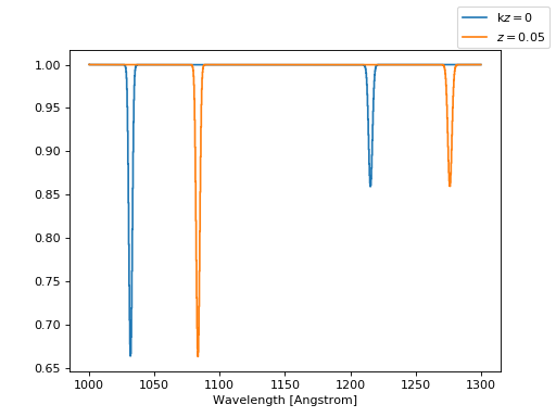
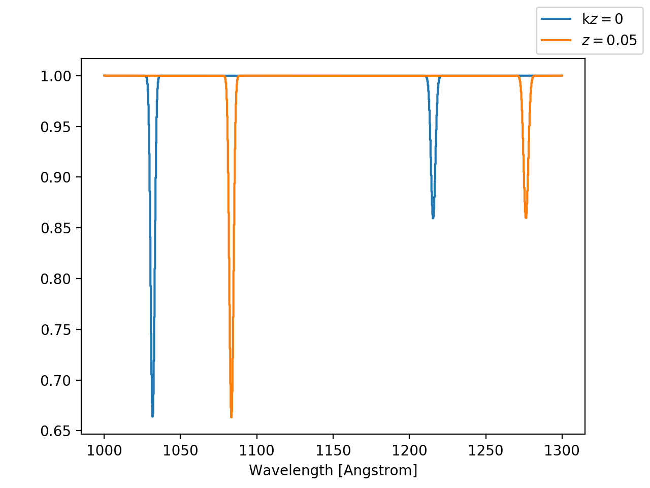
Implementing redshift
When creating a Spectral1D
model, the user can provide a redshift at which the output spectrum will
deposit the lines by including a z parameter.
Note
When fitting, including the z parameter
indicates the redshift of the input dispersion. Spectacle will de-redshift
the data input using this value before performing any fits. Also, the
provided continuum is not included in redshifting.
>>> from astropy import units as u
>>> import numpy as np
>>> from matplotlib import pyplot as plt
>>> from spectacle.modeling import Spectral1D, OpticalDepth1D
>>> line1 = OpticalDepth1D("HI1216", v_doppler=500 * u.km/u.s, column_density=14)
>>> line2 = OpticalDepth1D("OVI1032", v_doppler=500 * u.km/u.s, column_density=15)
>>> spec_mod = Spectral1D([line1, line2], continuum=1, z=0, output='flux')
>>> spec_mod_with_z = Spectral1D([line1, line2], continuum=1, z=0.05, output='flux')
>>> x = np.linspace(1000, 1300, 1000) * u.Unit('Angstrom')
>>> f, ax = plt.subplots()
>>> ax.step(x, spec_mod(x), label="k$z=0$")
>>> ax.step(x, spec_mod_with_z(x), label="$z=0.05$")
>>> ax.set_xlabel("Wavelength [Angstrom]")
>>> f.legend(loc=0)
(Source code, png, hires.png, pdf)