Fitting

The core Spectral1D behaves exactly like an Astropy model and can be used with any of the supported non-linear Astropy fitters, as well as some not included in the Astropy library.

Spectacle provides a default Levenberg–Marquardt fitter in the CurveFitter class.

>>> from spectacle.fitting import CurveFitter
>>> from spectacle.modeling import Spectral1D, OpticalDepth1D
>>> import astropy.units as u
>>> from matplotlib import pyplot as plt
>>> import numpy as np

Generate some fake data to fit to:

>>> line1 = OpticalDepth1D("HI1216", v_doppler=10 * u.km/u.s, column_density=14)
>>> spec_mod = Spectral1D(line1, continuum=1, output='flux')
>>> x = np.linspace(-200, 200, 1000) * u.Unit('km/s')
>>> y = spec_mod(x) + (np.random.sample(1000) - 0.5) * 0.01

Instantiate the fitter and fit the model to the data:

>>> fitter = CurveFitter()
>>> fit_spec_mod = fitter(spec_mod, x, y)

Users can see the results of the fitted spectrum by printing the returned model object

>>> print(fit_spec_mod)  
Model: Spectral1D
Inputs: ('x',)
Outputs: ('y',)
Model set size: 1
Parameters:
    amplitude_0 z_1 lambda_0_2 f_value_2   gamma_2      v_doppler_2      column_density_2      delta_v_2          delta_lambda_2    z_4
                     Angstrom                              km / s                                km / s              Angstrom
    ----------- --- ---------- --------- ----------- ------------------ ------------------ ------------------ --------------------- ---
            1.0 0.0  1215.6701    0.4164 626500000.0 10.010182187404824 13.998761432240995 1.0052009119192702 -0.004063271434522016 0.0

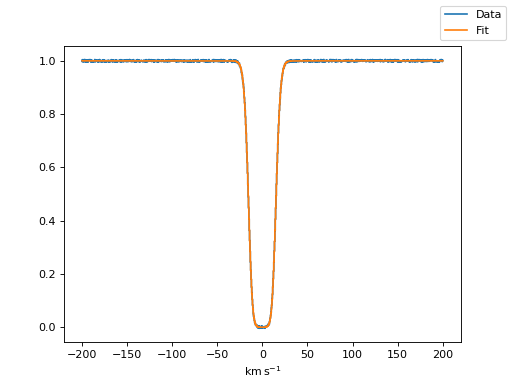
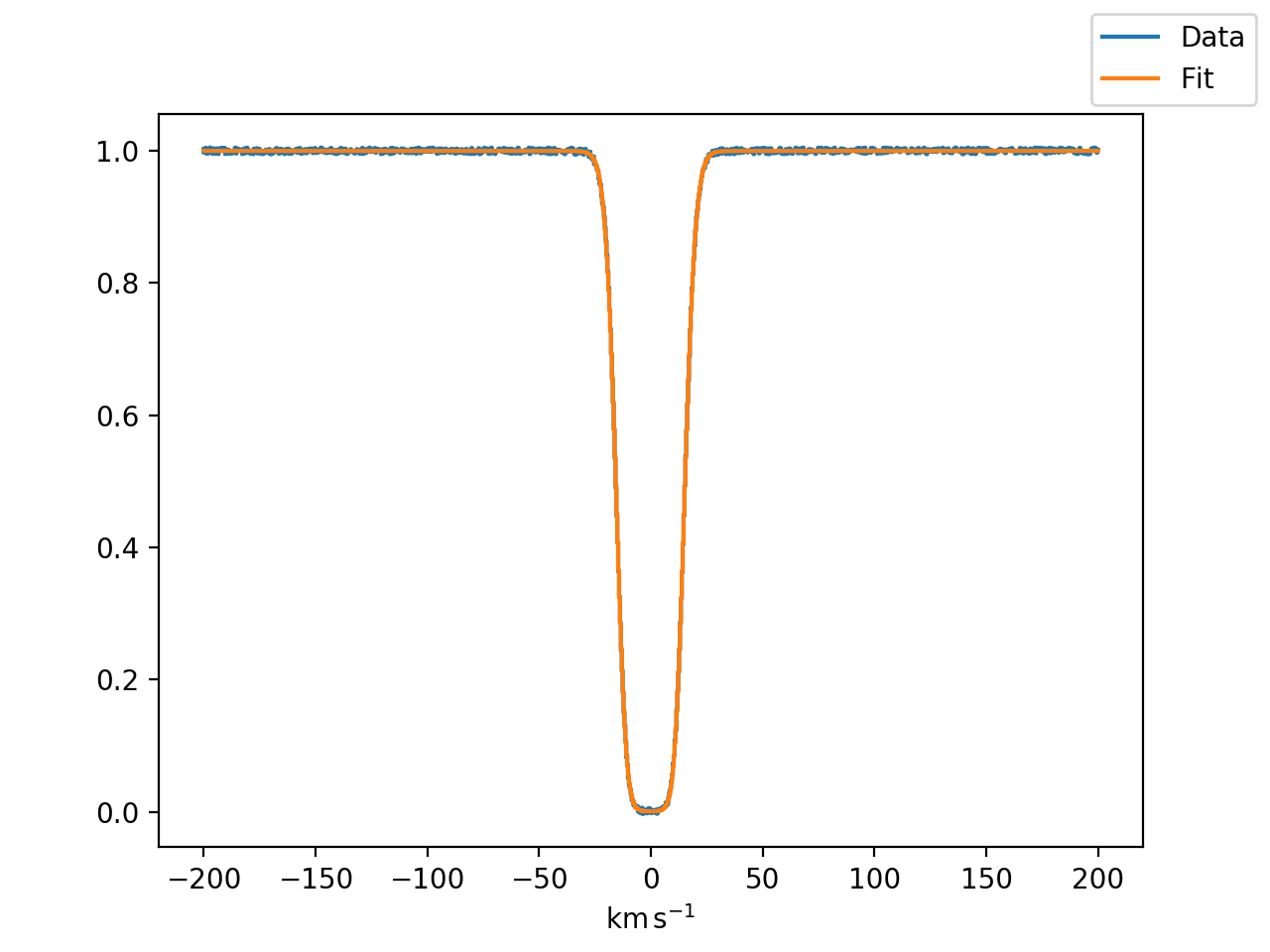
Plot the results:

>>> f, ax = plt.subplots()  
>>> ax.step(x, y, label="Data")  
>>> ax.step(x, fit_spec_mod(x), label="Fit")  
>>> f.legend()  

(Source code, png, hires.png, pdf)

On both the CurveFitter class and the EmceeFitter class described below, parameter uncertainties can be accessed through the uncertainties property of the instantiated fitter after the fitting routine has run.

>>> fitter.uncertainties  
    <QTable length=9>
      name               value                  uncert          unit
     str16              float64                float64         object
---------------- ---------------------- --------------------- --------
             z_0                    0.0                   0.0     None
      lambda_0_1              1215.6701                   0.0 Angstrom
       f_value_1                 0.4164                   0.0     None
         gamma_1            626500000.0                   0.0     None
     v_doppler_1     10.000013757295898  0.000957197044912263   km / s
column_density_1     14.000043173540684 3.589807779429899e-05     None
       delta_v_1 0.00011598087488537782 0.0006777042342563724   km / s
  delta_lambda_1                    0.0                   0.0 Angstrom
     amplitude_2                    1.0                   0.0     None

Using the MCMC fitter

Spectacle provides Bayesian fitting through the emcee package. This is implemented in the EmceeFitter class. The usage is similar above, but extra arguments can be provided to control the number of walkers and the number of iterations.

from spectacle.fitting import EmceeFitter
...

fitter = EmceeFitter()
fit_spec_mod = fitter(spec_mod, x, y, , nwalkers=250, steps=100, nprocs=8)

The fitted parameter results are given as the value at the 50th quantile of the distribution of walkers. The uncertainties on the values can be obtained through the uncertainties property on the fitter instance, and provide the 16th quantile and 80th quantile for the lower and upper bounds on the value, respectively.

Note

The MCMC fitter is a work in progress. Its results are dependent on how long the fitter runs and how many walkers are provided.

Custom fitters with the line finder

The LineFinder1D class can also be passed a fitter instance if the user wishes to use a specific type. If no explicit fitting class is passed, the default CurveFitter is used. Fitter-specific arguments can be passed into the fitter_args keyword as well.

line_finder = LineFinder1D(ions=["HI1216", "OVI1032"], continuum=0,
                           output='optical_depth', fitter=LevMarLSQFitter(),
                           fitter_args={'maxiter': 1000})

More information on using the line finder can be found in the line finding documentation.