Analysis

Spectacle comes with several statistics on the line profiles of models. These can be accessed via the line_stats() method on the spectrum object, and will display basic parameter information such as the centroid, column density, doppler velocity, etc. of each line in the spectrum.

Three additional statistics are added to this table as well: the equivalent width (ew), the velocity delta covering 90% of the flux value (dv90), and the full width half maximum (fwhm) of the feature.

>>> spec_mod.line_stats(x)  

<QTable length=2>
  name     wave   col_dens  v_dop  delta_v delta_lambda          ew                dv90                fwhm
         Angstrom           km / s  km / s   Angstrom         Angstrom            km / s             Angstrom
bytes10  float64  float64  float64 float64   float64          float64            float64             float64
------- --------- -------- ------- ------- ------------ ------------------- ------------------ --------------------
 HI1216 1215.6701     13.0     7.0     0.0          0.0 0.05040091274475814  15.21521521521521 0.048709144294889484
 HI1216 1215.6701     13.0    12.0    30.0          0.0 0.08632151159859157 26.426426426426445  0.08119004034051613

The dv90 statistic is calculated following the “Velocity Interval Test” formulation defined in Prochaska & Wolf (1997). In this case, the optical depth of the profile is calculated in velocity space, and 5% of the total is trimmed from each side, leaving the velocity width encompassing the central 90%.

Arbitrary line region statistics

It is also possible to perform statistical operations over arbitrary absorption or emission line regions. Regions are defined as contiguous portions of the profile beyond some threshold.

>>> from spectacle.modeling import Spectral1D, OpticalDepth1D
>>> import astropy.units as u
>>> from matplotlib import pyplot as plt
>>> import numpy as np
>>> from astropy.visualization import quantity_support
>>> quantity_support()  

We’ll go ahead and compose a spectrum in velocity space of two HI line profiles, with one offset by \(30 \tfrac{km}{s}\).

>>> line1 = OpticalDepth1D(lambda_0=1216 * u.AA, v_doppler=7 * u.km/u.s, column_density=13, delta_v=0 * u.km/u.s)
>>> line2 = OpticalDepth1D("HI1216", delta_v=30 * u.km/u.s,  v_doppler=12 * u.km/u.s, column_density=13)

>>> spec_mod = Spectral1D([line1, line2], continuum=1, output='flux')

>>> x = np.linspace(-200, 200, 1000) * u.km / u.s
>>> y = spec_mod(x)

Now, print the statistics on this absorption region.

>>> region_stats = spec_mod.region_stats(x, rest_wavelength=1216 * u.AA, abs_tol=0.05)
>>> print(region_stats)   
    region_start        region_end     rest_wavelength          ew                dv90               fwhm
       km / s             km / s           Angstrom          Angstrom            km / s            Angstrom
------------------- ------------------ --------------- ------------------- ----------------- --------------------
-12.612612612612594 48.648648648648674          1216.0 0.12297380252108686 46.44644644644646 0.056842794376279926

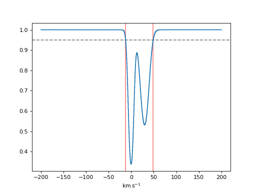
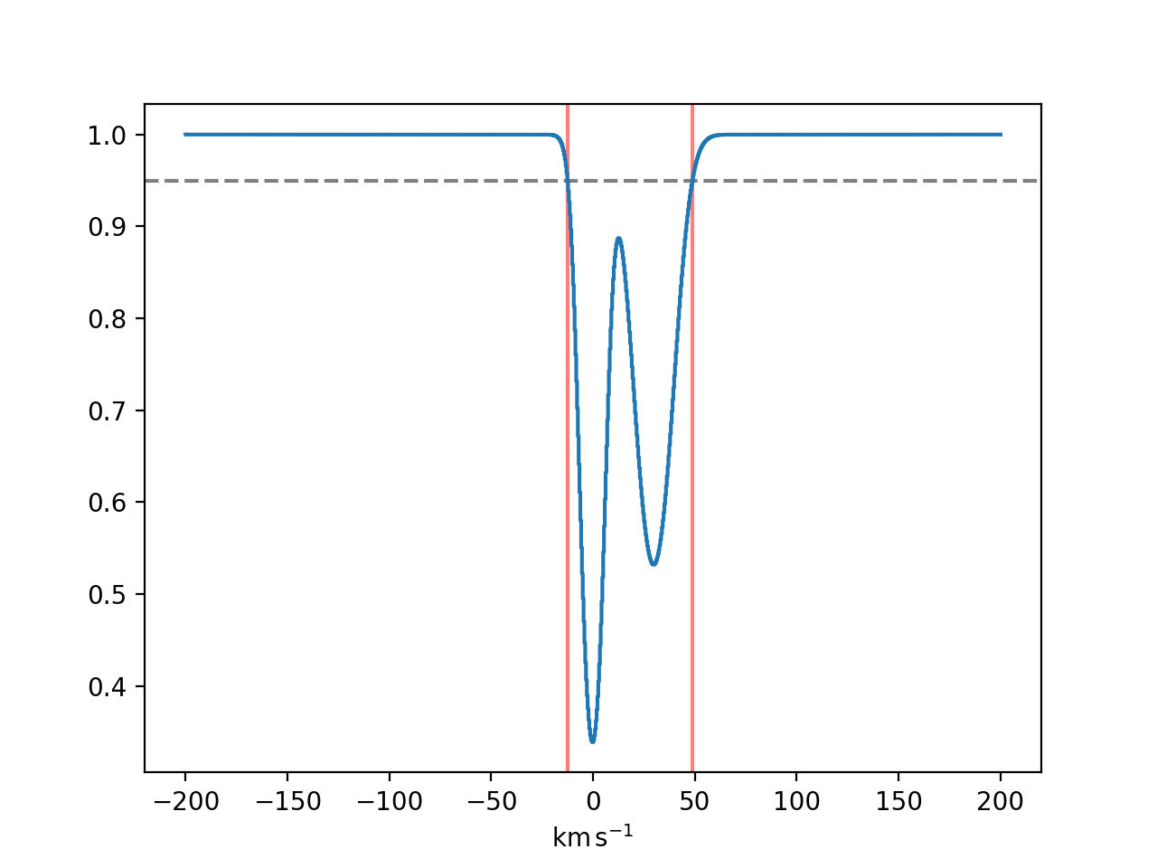
Plot to show the found bounds of the contiguous absorption region.

>>> f, ax = plt.subplots()  
>>> ax.axhline(0.95, linestyle='--', color='k', alpha=0.5)  
>>> for row in region_stats:
...    ax.axvline(row['region_start'].value, color='r', alpha=0.5)  
...    ax.axvline(row['region_end'].value, color='r', alpha=0.5)  
>>> ax.step(x, y)  

(Source code, png, hires.png, pdf)

Re-sampling dispersion grids

Spectacle provides a means of doing flux-conversing re-sampling by generating a re-sampling matrix based on an input spectral dispersion grid and a desired output grid.

>>> from spectacle.modeling import Spectral1D, OpticalDepth1D
>>> from spectacle.analysis import Resample
>>> import astropy.units as u
>>> from matplotlib import pyplot as plt
>>> import numpy as np
>>> from astropy.visualization import quantity_support
>>> quantity_support()  

Create a basic spectral model.

>>> line1 = OpticalDepth1D("HI1216")
>>> spec_mod = Spectral1D(line1)

Define our original, highly-sampled dispersion grid.

>>> vel = np.linspace(-50, 50, 1000) * u.km / u.s
>>> tau = spec_mod(vel)

Define a new, lower-sampled dispersion grid we want to re-sample to.

>>> new_vel = np.linspace(-50, 50, 100) * u.km / u.s

Generate the resampling matrix and apply it to the original data.

>>> resample = Resample(new_vel)
>>> new_tau = resample(vel, tau)

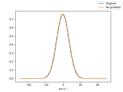
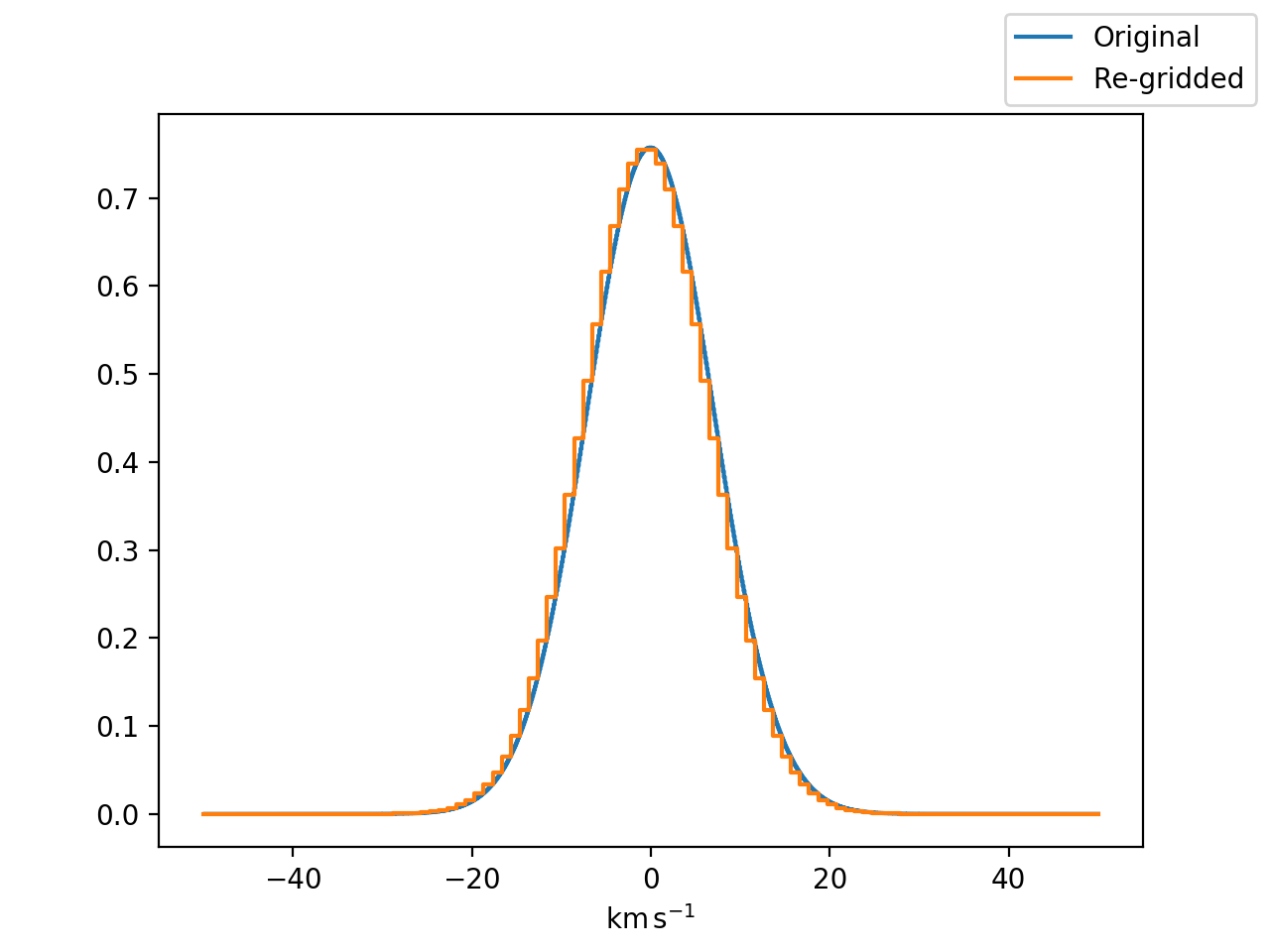
Plot the results.

>>> f, ax = plt.subplots()  
>>> ax.step(vel, tau, label="Original")  
>>> ax.step(new_vel, new_tau, label="Re-gridded")  
>>> f.legend()  

(Source code, png, hires.png, pdf)